Calibration in Binary outcomes
Definition
Calibration describs the agreement between observed outcomes and predictions. The most common definition of calibration is that if we observe p% risk among patients with a predicted risk of p%. So, if we predict 70% probability of residual tumor tissue for a testicular cancer patient, the observed frequency of tumor should be approximately 70 out of 100 patients with such a predicted probability.
Methods
Calibration Plot
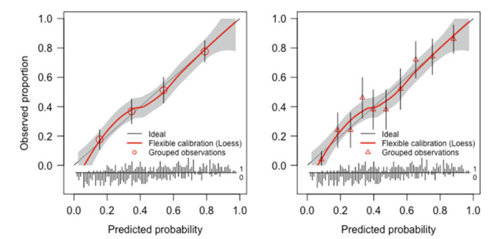
A calibration plot has predictions on the x-axis, and the outcome on the y-axis. A line of identity helps for orientation: perfect predictions should be at the 45° line.
For binary outcomes, the plot contains only 0 and 1 values for the y-axis. Such probabilities are not observed directly. Smoothing techniques can be used to estimate the observed probabilities of the outcome (p(y = 1)) in relation to the predicted probabilities. The observed 0/1 outcomes are replaced by values between 0 and 1 by combining outcome values of subjects with similar predicted probabilities. using the loess algorithm. Confidence intervals can be calculated for such a smooth curve.
If we plot observed outcome in groups defined by quintile or by decile of predictions. This makes the plot a graphical illustration of the Hosmer–Lemeshow goodness-of-fit test.

Left and right panels only differ in the number of groups (4 vs 10)
Test
Hosmer-Lemeshow test
The Hosmer-Lemeshow test is computed by partitioning the study population into k groups based on the predicted probability of an event obtained from the risk prediction model (usually k=10).
A chi-square statistic is then used to compare the observed and expected events. When assessing the calibration of a risk score using the data set it was developed on, one degree of freedom is lost in defining the groups, so the chi-square statistic is assessed using k-2 degrees of freedom. When assessing calibration on a new data set, this is not a problem and k-1 degrees of freedom are used for the chi-square test. Limitations of the Hosmer-Lemeshow test are well-known and include its dependence on arbitrary groupings of patients, poor power in small data sets, as well as the fact that it only results in a p-value.
In the idea of model-based framework for calibration, Hosmer-Lemeshow test equals to test \(\gamma_1 = \gamma_2 = ... = \gamma_k = 0\) in the regression model as below:
\[ logit(E(Y)) = \gamma_1 grpup_1 + \gamma_2 grpup_2 + ... + \gamma_k grpup_k + p \] wherein, \(group_1\), \(group_2\), … \(group_k\) are dummy variables; \(p\) is the linear predictor.
Calibration-in-the-large
Calibration-in-the-large is a basic measure of agreement between the observed and predicted risks, which is computed as the difference between the mean observed risk and the mean predicted risk. The mean observed and predicted risks will definitely agree when assessed in the data set used to build the risk model, but agreement is less certain when applying a risk score to a new data set.
In the model based framework point of view, it is equal to test \(\gamma_0 = 0\) in the following model.
\[ logit(E(Y)) = \gamma_0 + p \]
Calibration slope
The calibration slope, which is calculated by regressing the observed outcome on the predicted probabilities, does not suffer from the limitations of the Hosmer-Lemeshow test, as it does not require grouping patients and the estimated slope obtained from the regression model provides a measure of effect size and a confidence interval, in addition to a p-value. For these reasons, the calibration slope is more informative and is the preferred method for assessing calibration. It might be more prevalent were it not for the prominence of the Hosmer-Lemeshow test in many statistical packages.
In the calibration model,
\[
logit(E(Y)) = \gamma_0 + \gamma_1 p
\]
it equals test \(\gamma_1 = 1\).
hierarchy of calibration levels
| Level | Definition | Assessment |
|---|---|---|
| Mean | Observed event rate equals average predicted risk |
calibration-in-the-large test (df = 1): a(given b = 1) = 0 |
| Weak | No systematic over-fitting or under-fitting and/or overestimation or underestimation of risks |
calibration-in-the-large and calibration slope: test (df = 2) a(given b = 1) = 0 and b = 1 |
| Moderate | Predicted risks correspond to observed event rates |
calibration plot (e.g. loess or splines), or grouped predictions (including Hosmer-Lemeshow test) |
| Strong | Predicted risks correspond to observed event rates for each and every covariate pattern |
Scatter plot of predicted risk and observed event rate per covariate pattern; impossible when continuous predictors are involved |
Reference:
Steyerberg EW. Clinical Prediction Models: A Practical Approach to Development, Validation and Updating. New York: Springer; 2019
Crowson CS, Atkinson EJ, Therneau TM. Assessing calibration of prognostic risk scores. Statistical methods in medical research. 2016 Aug;25(4):1692-706.
Van Calster B, Nieboer D, Vergouwe Y, De Cock B, Pencina MJ, Steyerberg EW. A calibration hierarchy for risk models was defined: from utopia to empirical data. Journal of clinical epidemiology. 2016 Jun 1;74:167-76.
Austin PC, Steyerberg EW. Graphical assessment of internal and external calibration of logistic regression models by using loess smoothers. Statistics in medicine. 2014 Feb 10;33(3):517-35.